Selecting data from a drop-down list is a convenient and accurate way of entering data into a range. It helps in ensuring that the correct data is entered quickly in Microsoft  Excel. However, a slicer provides a quicker, better and easier way of selecting data from a list. In this tip, we explain how to use a slicer to select data from an Excel range. Slicers are also used for interactively filtering data in a Pivot Table or other table. In the below example, you can see that we have a drop-down list from which to select different months. You are welcome to download the workbook to practice. Applies to: Microsoft  Excel  2010, 2013 and 2016.
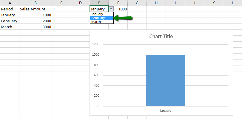
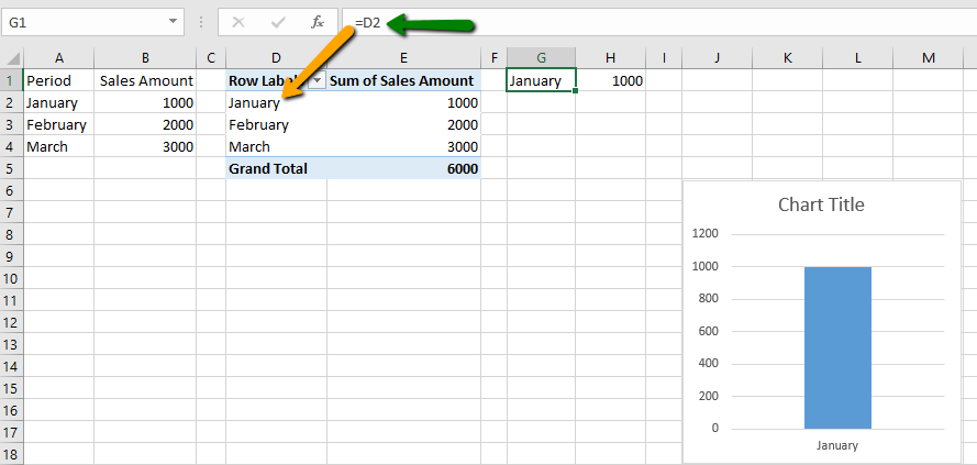
There is nothing wrong with this method, however with one extra step, we can make flipping between these months quicker. We have introduced a Pivot Table created from the same data range. In cell E1, we have deleted the data list and then referenced the first row of the Pivot Table in cell G1 and H1, which is showing January in this example.
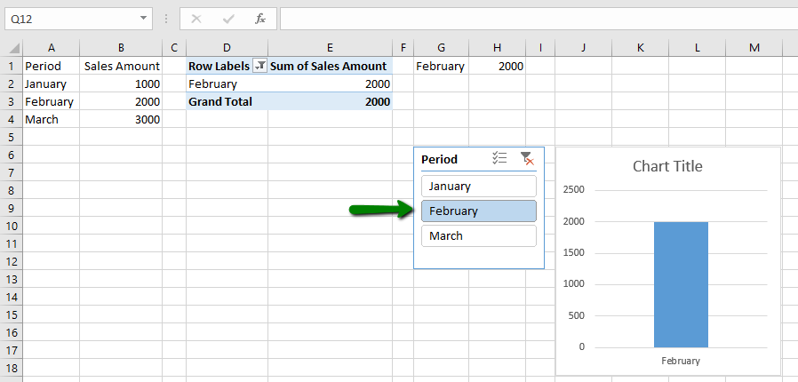
The last step is to simply insert a slicer on that Pivot Table. To create a slicer, select any cell within the Pivot Table, and then select the Insert Tab, and Slicer under the Filters group.
Now you can click on the slicer for the month you want to see, rather than having to click on a drop-down list.
By using this method, time will be saved as the months are easily and quickly selected.