Have you ever wanted to personalize your chart headings to further enhance the user’s report experience? In this tip we will show you how to customize chart titles according to the filter chosen.
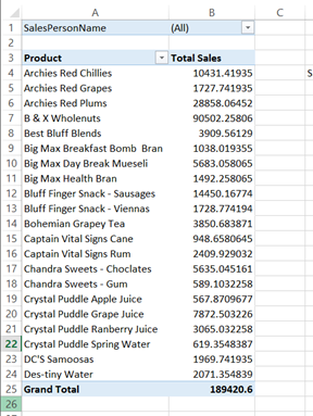
- I have a simple report that displays a PivotTable with the Total Sale by Product and a filter by sales person name.
- Next, I insert a chart by clicking within the PivotTable, selecting the Insert Tab in the ribbon then selecting the Recommended Charts button and then choosing the chart I like. Once that is done, notice the Chart Title can be edited.

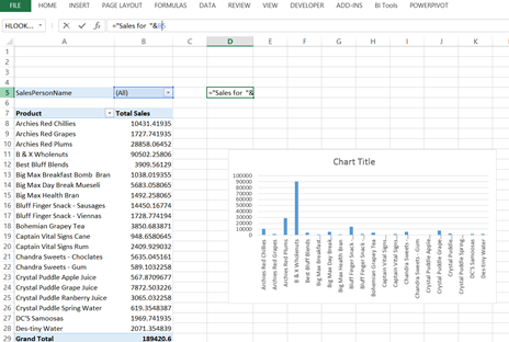
- I want the chart to reflect what I choose in the Sales Person Name filter. To do this, I first create a formula anywhere on the sheet, preferably out of sight that references the title and the filter. First, click into the Formula bar and type equals and the formula as follows: =”Sales for “&B5. The quotation marks represent the text to display in the title. The ampersand (&) connects the text (title) string with the cell reference which is B5 or the filter result.
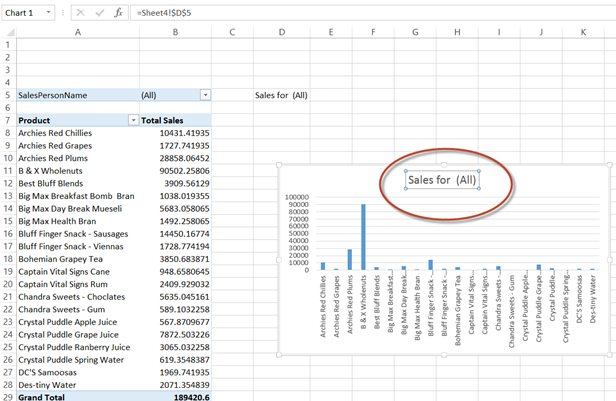
- Next, click on the Chart Title – not the text, the title box only. Then, within the formula bar type equals (=) and click on the cell with the new formula and press enter. You should see the title with (All) represented. Next, select a salesperson from the filter and see how the Chart Title dynamically changes depending on the filter chosen.
No filter used:
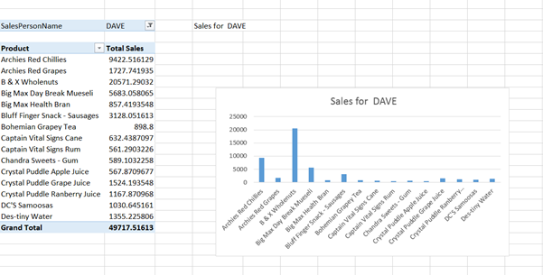
DAVE chosen from filter